Spruce Overview
Introduction
Spike-sorting is the process of taking electrophysiological data, expressed as a set of voltage time series from one or more probes, and separating the observed spikes into categories associated with different neural units. In recent years, probe technology has significantly improved the density and number of channels that can be recorded simultaneously, vastly increasing the quantity of data available for spike-sorting, making good automatic spike-sorting algorithms a key bottleneck for progress in neuroscience.
Unfortunately, development of quality spike-sorting algorithms is hampered by the relative lack of ground-truth data on which to evaluate them. The data used here, collected by the Synthetic Neurobiology Group at MIT, provide a new opportunity to do detailed comparative analyses. In particular, while existing databases like SpikeForest focus on comparing algorithms to one another for benchmarking, the Spruce project focuses on examining what data criteria are important for the proper algorithm functioning. We are interested in answering questions like: What is the point where increasing channel count or electrode density is no longer useful? What type of noise is most harmful to effective spike-sorting performance? Which algorithms are more or less robust to which kinds of factors?
Methodology
The Synthetic Neurobiology Group collected 51 recordings of neural activity in the primary visual cortex of mice, using multi-channel probes with between 50 and 256 electrodes in conjunction with an intracellular patch on a single neuron. (Each channel is the signal from a single electrode.) Spikes were identified from the intracellular recordings and spike times were recorded according to the peaks of the derivative of the voltage. If spikes were within 20ms of each other, they were labeled as part of a burst. Twelve of the recordings had mean extracellular spike amplitudes larger than 50 μV, and were selected for further analysis. Initial work involved a simple threshold-based spike detection algorithm, and analyzing the ampltiude distribution of spikes without taking into account their shape. (For more details about the data collection and initial analysis, see the paper, “Automated in vivo patch clamp evaluation of extracellular multielectrode array spike recording capability”.)
Real-world spike sorting applications, however, use more sophisticated algorithms, and we are interested in investigating what conditions cause these algorithms to succeed or fail. The three algorithms we used for subsequent analysis are:
Kilosort, released in 2016 from UCL’s Cortex Lab, uses an iterative template matching procedure, with a single “template” waveform corresponding to each cluster. The data is processed sequentially, with each batch containing a “template matching” step to detect and extract spike times followed by an “inference” step to adjust the template set. The entire dataset is run through multiple times until the total cost function converges, but the template set (of a fixed size) is allowed to vary over the course of the dataset to account for probe drift. In the final pass through the data, template subtraction is used to find overlapping spikes.
Kilosort2, an update to Kilosort, has two key changes. The first is that the batches within the data are reordered before any processing, to make non-monotonic drift more monotonic. The second is that template subtraction is used in every pass through the data, with a variable number of templates growing or shrinking according to unaccounted-for spikes, rather than only at the end. Other changes include a more sophisticated check for merges and splits in a final pass.
MountainSort4 uses a single initial detection step by finding spatiotemporal peaks, placing all events in a single cluster per electrode, followed by an iterative splitting algorithm (ISO-SPLIT). Clusters from different electrodes are compared to eliminate duplicates, and then waveform subtraction is used to eliminate events that are duplicated across multiple clusters.
All three algorithms use similar preprocessing steps, generally consisting of a bandpass filter and a ZCA-like spatial whitening step. There are minor differences, however. (For instance, MountainSort4 includes a noise elimination step by removing outlier frequency bands, Kilosort includes a common average reference, and Kilosort2 uses geometry information in its spatial whitening.)
All three algorithms have some number of parameters that could be tuned, but for the sake of a fair comparison, we used the default parameters for all algorithms so we could treat them as black boxes. (The number of clusters to output in Kilosort, which is meant to vary with the number of channels and so has no well-defined default value, was set to the smallest multiple of 32 larger than twice the number of channels.)
In order to explore the effects of probe density and size on spike-sorting performance, we took a subset of the channels (a “channel cut”) in an extracellular recording as the input for any given run, and varied that subset to conduct experiments. The procedure for selecting the channel cut, similar to the procedure used in the paper, went as follows:
Sort the channels according to their mean spike amplitude, from highest to lowest. This ensures that the starting electrodes are the ones closest to the patched unit.
Proceed down the list, taking electrodes according to the specified density, until the specified number are selected. If a given experiment called for a density of 1/3 of the original electrode density, for instance, then 1 channel from the top 3 would be taken, followed by 1 channel from the next 3, followed by 1 from the next 3, et cetera, continuing until enough channels were selected.
For each pairing of an algorithm and a channel cut, we ran multiple spike-sorting trials, to account for random variation in the results due to seeding.
We developed a variety of metrics for the performance of a run, detailed in the data inspector glossary, as well as two tools (the data inspector and the aggregate viewer) for visualizing them. Nearly all figures displayed below can be created using one of the two tools. The most commonly-used metric was F1 score, a combination of cluster precision and cluster recall. Since the ground truth patch data only refers to a single neuron, the metrics evaluate the sorting algorithm’s performance at separating out the cluster of spikes associated with that neuron, and do not evaluate the algorithm’s performance at sorting internally between any other events.
Results
Recording |
Mouse |
Layer |
# of Working Electrodes |
All Spikes |
Burst Spikes |
MAD, μV |
Mean Nonburst Amplitude, μV |
Other Deflections in Spike Range |
Portion of Burst Spikes Between 2 and 6 MAD |
Mean F1-Score (KS, 32-Channel) |
Mean F1-Score (KS2, 32-Channel) |
Mean F1-Score (MS4, 32-Channel) |
|---|---|---|---|---|---|---|---|---|---|---|---|---|
1 |
A |
5 |
236 |
3877 |
989 |
14 |
-267 |
36 |
0.27 |
0.79 |
0.93 |
0.84 |
2 |
B |
5 |
122 |
2372 |
969 |
7 |
-100 |
2720 |
0.06 |
0.84 |
0.86 |
0.46 |
3 |
C |
5 |
236 |
323 |
15 |
8 |
-91 |
766 |
0.07 |
0.56 |
0.61 |
0.23 |
4 |
D |
5 |
214 |
2926 |
1328 |
9 |
-77 |
370 |
0.46 |
0.81 |
0.91 |
0.65 |
5 |
B |
5 |
122 |
8748 |
4004 |
9 |
-82 |
8441 |
0.23 |
0.74 |
0.87 |
0.42 |
6 |
E |
2/3 |
58 |
1136 |
291 |
9 |
-69 |
262 |
0.18 |
0.95 |
0.97 |
0.84 |
7 |
F |
5 |
225 |
4640 |
1625 |
13 |
-68 |
37073 |
0.70 |
0.77 |
0.05 |
0.17 |
8 |
B |
2/3 |
122 |
823 |
93 |
6 |
-64 |
11 |
0.00 |
0.98 |
0.99 |
0.89 |
9 |
G |
2/3 |
238 |
205 |
6 |
6 |
-60 |
1725 |
0.17 |
0.68 |
N/A |
0.02 |
10 |
B |
2/3 |
122 |
78 |
16 |
6 |
-57 |
4 |
0.06 |
0.84 |
0.97 |
0.01 |
11 |
F |
5 |
225 |
2976 |
1199 |
8 |
-53 |
20907 |
0.55 |
0.76 |
0.03 |
0.08 |
12 |
D |
2/3 |
214 |
1592 |
216 |
8 |
-52 |
3928 |
0.30 |
0.81 |
0.65 |
0.11 |
The table above (a subset of the properties listed in the data collection paper, combined with some result statistics) displays the hetereogeneity between the different recordings. Although there are clear differences in quality, the recordings cannot be unambiguously lined up from “best” to “worst”, as the ones with the strongest spikes are not always the ones with the quietest background signal, or the ones with the most well-behaved spike amplitude distribution. It seems that poor spike-sorting performance is most correlated with “other deflections in spike range” (the spike range being anything higher than one standard deviation below the mean spike amplitude). Notably, spike-sorting performance is only weakly correlated with signal-to-noise ratio - sometimes a low SNR comes from a large number of small background fluctuations, but sometimes it comes from a smaller number of larger fluctuations.
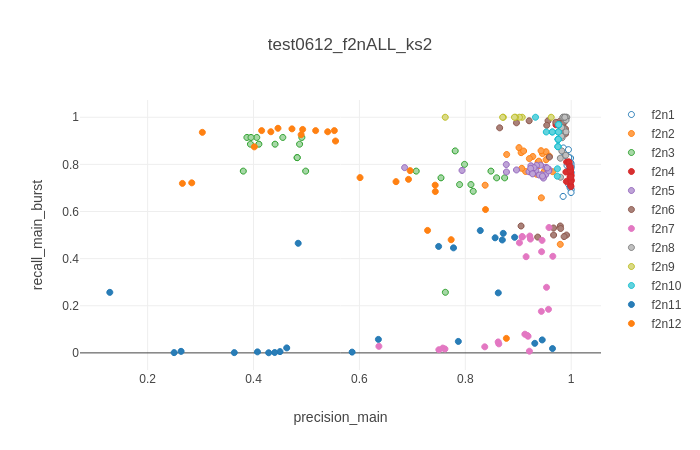
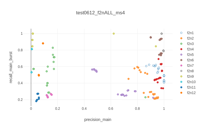
Scatter plot of two key metrics, colored by dataset, for two different algorithms (top: Kilosort2. bottom: MountainSort4.) Each dataset was used for 24 trials, split between three different channel cuts (8 trials with the top 32 channels, 8 trials with half of the top 58, and 8 trials with all of the top 58).
The above figures further underscore the amount to which the results of spike-sorting are highly variable and strongly idiosyncratic to the dataset and algorithm used. For instance, the runs of Kilosort2 on recording #4 (f2n4) are very tight and consistent - but the runs of Kilosort2 on #2 or #11 span are highly variable in both precision and recall, and the runs of MountainSort4 on recordings #5 or #7 are strongly clustered into three clumps representing the three different channel cuts. It generally seems that MountainSort4 is more deterministic than either of the Kilosorts, and that Kilosort is more resilient to bad or poorly-cut data than Kilosort2, but for more specific trends, we must examine each recording individually.
Example: Kilosort on recording 11

Aggregate view of the F1 scores from running Kilosort on recording 11, across a variety of trials and channel cuts. Densities and channel counts are slightly dithered on this plot for visibility.
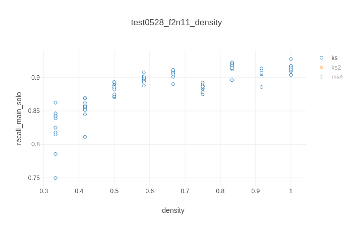
Batch inspector view of the recalls from running Kilosort on recording 11, with a sweep of channel cuts of varying densities, but the total number of channels held constant at 60.
Kilosort’s performance on recording #11, a low-SNR dataset that KiloSort2 and MountainSort4 struggle with, depends most strongly on channel count. If there are 50 or more channels, as shown above, it performs well, with F1 scores around 0.8, precisions around 0.95, and recalls around 0.9/0.55 (solo/burst). Having those channels be more densely packed around the highest-magnitude electrode helps slightly, primarily in recall by about 5%. But if there are fewer than 50 channels, F1 scores decline rapidly, due to both declining precision and declining recall.
More Summaries
Using the same kind of investigation as done for the example above, we observe the following trends on the datasets for which experiments were conducted using a variety of channel cuts (recordings #1, #2, #3, #11, #12):
Recording |
Algorithm |
Functional? |
To what extent? |
Best under what conditions? |
Can you further improve? |
|---|---|---|---|---|---|
f2n1 |
KS |
Yes |
f1 ~= 0.8 |
density > 1/6 |
not really |
f2n1 |
KS2 |
Yes |
f1 ~= 0.95 |
channels > 15 |
more density helps |
f2n1 |
MS4 |
Yes |
f1 ~= 0.9 |
density ~= 2/3 |
more channels helps |
f2n2 |
KS |
Yes |
f1 ~= 0.85 |
channels > 40 |
not really |
f2n2 |
KS2 |
Yes |
f1 ~= 0.9 |
channels > 50 |
not really |
f2n2 |
MS4 |
Yes |
f1 ~= 0.7 |
density ~= 1/2 |
fewer channels helps |
f2n3 |
KS |
Noisy |
f1 ~= 0.6 |
density >= 1/6 |
more channels helps |
f2n3 |
KS2 |
Noisy |
f1 ~= 0.7 |
density > 1/2 |
fewer channels helps |
f2n3 |
MS4 |
Not really |
f1 ~= 0.25 |
density > 1/2 |
more density helps |
f2n11 |
KS |
Yes |
f1 ~= 0.8 |
channels > 50 |
more density helps |
f2n11 |
KS2 |
Noisy |
f1 <= 0.8 |
extent > 100 |
density ~= 0.5 helps |
f2n11 |
MS4 |
No |
f1 ~= 0.2 |
density < 1/3 |
fewer channels helps |
f2n12 |
KS |
Yes |
f1 ~= 0.8 |
density ~= 2/3 |
not really |
f2n12 |
KS2 |
Yes |
f1 ~= 0.6 |
channels > 50 |
density ~= 2/3 helps |
f2n12 |
MS4 |
No |
f1 < 0.2 |
density < 1/3 |
not really |
Conclusions
A few broad patterns can be observed.
The most striking is that MountainSort4’s performance is strongly dependent on electrode density, to almost the exclusion of overall channel count as a parameter. As density increases, recall always decreases, and precision either significantly increases (in the higher-performance datasets) or significantly decreases (in the lower-performance datasets). This may be because MountainSort4 identifies candidate spiking events with a single channel, and uses a relatively strict maximum-on-neighbors criterion to merge candidates. In the presence of noise, this policy may fail to properly deduplicate, to an extent strongly influenced by the number of neighbors each electrode has. By contrast, Kilosort and KiloSort2 identify candidate events with a time interval over all channels, making their classification more likely to be influenced by the inclusion of electrodes far from the ground truth unit.
Another pattern is that both Kilosort and KiloSort2 tend to have a “plateau” of performance, that is, there is a minimum amount of information they need to function properly, but once they have it, providing more information is unlikely to significantly improve performance metrics. (If the algorithms are noisy - i.e. having a high variance between runs with identical channel cuts, depending on initialization - then providing more information may improve reliability, but it does not really improve peak performance.) This is intuitive in the case of adding more channels, but surprising in the case of increasing density; it suggests that errors in sorting are not due to imperfections in fitting the spike model to data, but imperfections in the spike model itself.
The third pattern is that while KiloSort2 has highly irregular performance on recordings #7, #11, and #12, Kilosort remains steady. On the other nine recordings, however, KiloSort2 generally performs significantly better than Kilosort, which remains steady. KiloSort2 seems to be a “high-risk, high-reward” improvement of Kilosort - its main added feature, drift correction through time reordering, can add important model flexibility if the data are clear enough to permit a reliable reordering, but can severely impair performance if not.
This is consistent with the observations on SpikeForest by Magland et al., who noted that KiloSort2 performs especially well on high-SNR datasets, and MountainSort4 thrives on low-channel-count datasets such as monotrodes and tetrodes.
Useful Links
SpikeForest is a reproducible, continuously-updating dashboard produced by the Flatiron Institute, which benchmarks the performance of many different spike sorting algorithms on many different datasets (some synthetic, some real).
http://scalablephysiology.org/mea_validation/ is the website for the first phase of the Spruce project, i.e. the data collection.
https://burstweb.herokuapp.com/, produced by Brian Allen, is a widget for visualizing the differences between what the traces of burst spikes look like and what the traces of non-burst spikes look like. It is based on the same dataset as this website.
Willow is a 1024-channel electrophysiology recording system used for the Spruce data collection.